Closed String Topologies
Tags
When calculating scattering amplitudes via the path integral, we must sum over all possible world-sheet topologies. To characterize the types of world-sheets that have to be considered at each level of its perturbative expansion, string theory makes use of the following theorem:
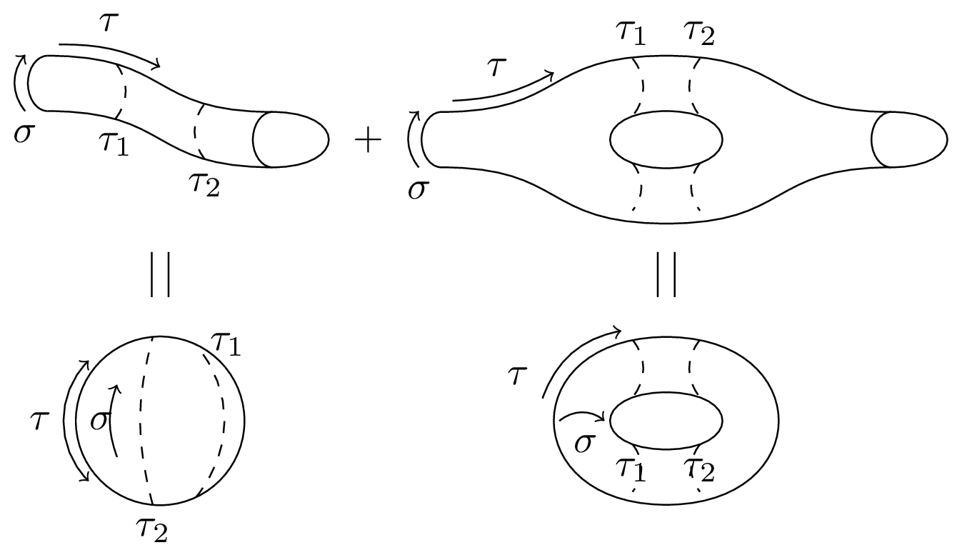
Every compact, connected, oriented two-dimensional manifold is topologically equivalent to a sphere with $g$ handles ($g$ for genus) and $b$ boundaries. A topological invariant of two-dimensional oriented surfaces is the Euler characteristic $\chi = 2 - 2g - b$.
What this boils down to is that we can obtain the topological characteristics of higher and higher loop-level world-sheet topologies by successively increasing in one-step increments the number of handles $g$ in case of the closed string and the number of boundaries $b$ for the open sector. This gives the topologies in this figure for the vacuum diagram of the closed sector up to one-loop level. For the open sector, see open string topologies.
Edit
Download
Code
closed-string-topologies.tex (114 lines)
\documentclass[tikz]{standalone}

\usetikzlibrary{tqft,calc}

\begin{document}

\begin{tikzpicture}[
    every tqft/.append style={
        transform shape, rotate=90, tqft/circle x radius=7pt,
        tqft/boundary separation=1cm, tqft/view from=incoming
      }
  ]

  % cobordism at upper left
  \pic[
    tqft/cylinder to prior,
    name=a,
    every incoming lower boundary component/.style={draw},
    every outgoing lower boundary component/.style={draw},
    cobordism edge/.style={draw},
  ];
  \pic[
    tqft/cup,
    cobordism edge/.style={draw},
    at=(a-outgoing boundary),
  ];

  % annotation of cobordism at upper left
  \coordinate (temp1) at ($(a-incoming boundary.west)!0.3!(a-outgoing boundary.west) +(0,0.08)$);
  \coordinate (temp2) at ($(a-incoming boundary.west)!0.7!(a-outgoing boundary.west) +(0,-0.08)$);
  \draw[dashed]
  (temp1) node[below] {$\tau_1$} to[bend right=40] ++(0,0.5)
  (temp2) node[below] {$\tau_2$} to[bend left=40] ++(0,0.5);
  \draw[->] ($(a-incoming boundary.west) - (0.2,0)$) node[below] {$\sigma$} to[bend left=40] ++(0,0.5);
  \draw (a-outgoing boundary) ++(0.85,0) node {$+$};
  \draw[->] ($(a-incoming boundary.east)+(0.1,0.1)$) to[bend left=13] +(0.9,-0.2);
  \node[above] at ($(a-incoming boundary.east)+(0.55,0.1)$) {$\tau$};

  % cobordism at upper right consisting of two 'pants' and a cup
  \pic[
    tqft/pair of pants,
    name=b,
    every incoming lower boundary component/.style={draw},
    cobordism edge/.style={draw},
    at={($(a-outgoing boundary)+(1.5,0)$)},
  ];
  \pic[
    tqft/reverse pair of pants,
    name=c,
    every outgoing lower boundary component/.style={draw},
    cobordism edge/.style={draw},
    at=(b-outgoing boundary 1),
  ];
  \pic[
    tqft/cup,
    cobordism edge/.style={draw},
    at=(c-outgoing boundary),
  ];

  % annotation of cobordism at upper right
  \draw[->] ($(b-incoming boundary.west) - (0.2,0)$) node[below] {$\sigma$} to[bend left=40] ++(0,0.5);
  \coordinate (temp1) at ($(b-between outgoing 1 and 2)!0.2!(c-between incoming 1 and 2) +(0,0.72)$);
  \coordinate (temp2) at ($(b-between outgoing 1 and 2)!0.8!(c-between incoming 1 and 2) +(0,0.72)$);
  \draw[dashed]
  (temp1) node[above] {$\tau_1$} to[bend left=40] +(0,-0.51) ++(0,-0.93) to[bend left=40] ++(0,-0.42)
  (temp2) node[above] {$\tau_2$} to[bend right=40] +(0,-0.51) ++(0,-0.93) to[bend right=40] ++(0,-0.42);
  \draw[->] ($(b-incoming boundary.east)+(0.1,0.1)$) to[bend right=13] +(0.9,0.25);
  \node[above] at ($(b-incoming boundary.east)+(0.5,0.2)$) {$\tau$};

  % drawing ring
  \pic[
    tqft ,
    name=d,
    incoming boundary components=0,
    outgoing boundary components=2,
    cobordism edge/.style={draw},
    anchor=between outgoing 1 and 2,
    at={($(b-between outgoing 1 and 2)!0!(c-between incoming 1 and 2) - (0,2.5)$)},
  ];

  \pic[
    tqft ,
    name=e,
    incoming boundary components=2,
    outgoing boundary components=0,
    cobordism edge/.style={draw},
    at = {(d-outgoing boundary 1)},
  ];
  \coordinate (temp1) at ($(d-between outgoing 1 and 2)!0.2!(e-between incoming 1 and 2) +(0,0.72)$);
  \coordinate (temp2) at ($(d-between outgoing 1 and 2)!0.8!(e-between incoming 1 and 2) +(0,0.72)$);
  \draw[dashed]
  (temp1) to[bend left=40] +(0,-0.51) ++(0,-0.93) node[below] {$\tau_1$} to[bend left=40] ++(0,-0.42)
  (temp2) to[bend right=40] +(0,-0.51) ++(0,-0.93) node[below] {$\tau_2$} to[bend right=40] ++(0,-0.42);

  \coordinate (temp1) at ($(d-between outgoing 1 and 2)!0.5!(e-between incoming 1 and 2)$);
  \coordinate (temp2) at (a-between first incoming and first outgoing);
  \draw[->] ($(e-incoming boundary 2)+(-1.1,-0.3)$) node[above left] {$\tau$} to[bend left=30] +(0.7,0.6);
  \draw [->] ($(d-between outgoing 1 and 2) + (-0.45,0)$) node [below right] {$\sigma$} to[bend left=40] +(0.4,0);
  \draw (temp1) ++(-0.075,1.5) -- ++(0,-0.4) ++(0.15,0) -- +(0,0.4);

  % drawing and annotating ball
  \node[draw, shape=circle, minimum width=1.5cm]
  at (temp1-|temp2) (circ) {};
  \draw[dashed] (circ) +(265:0.75) node[below] {$\tau_2$} to[bend left=15] +(95:0.75);
  \draw[dashed] (circ) +(295:0.75) to[bend right=40] +(65:0.75) node[right] {$\tau_1$};
  \draw[->] (circ) +(220:0.5) to[bend left=20] +(140:0.5);
  \node[right] at(circ.west) {$\sigma$};
  \draw (circ) ++(-0.075,1.5) -- ++(0,-0.4) ++(0.15,0) -- +(0,0.4);
  \draw[<->] (circ.south west) +(-0.1,0) to[bend left=45] ($(circ.north west)+(-0.1,0)$);
  \node[left=0.25em] at(circ.west) {$\tau$};
\end{tikzpicture}

\end{document}