Bose Einstein Distribution
Tags
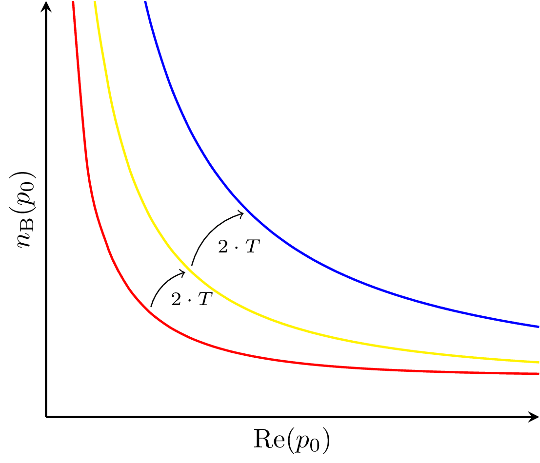
Illustrating the change in the real part of the Bose-Einstein distribution, i.e. the average occupancy of the ground state of a bosonic system, from doubling the temperature. Pulled from arxiv:1712.09863.
Edit
Download
Code
bose-einstein-distribution.tex (40 lines)
\documentclass{standalone}

\usepackage{pgfplots,mathtools}
\pgfplotsset{compat=newest}

\usetikzlibrary{intersections}

\let\Re\relax
\DeclareMathOperator{\Re}{Re}

\begin{document}
\begin{tikzpicture}
  \begin{axis}[
      domain = 0:2, ymax = 5,
      xlabel = $\Re(p_0)$,
      ylabel = $n_\text{B}(p_0)$,
      ticks=none, smooth,
      thick, axis lines = left,
      every tick/.style = {thick},
      width=8cm, height=7cm]

    \def\nB#1{1/(e^(x/#1) - 1) + 1/2}

    \addplot[name path=T1, color=red] {\nB{0.5}};

    \addplot[name path=T2, color=yellow] {\nB{1}};

    \addplot[name path=T3, color=blue] {\nB{2}};

    \addplot[draw=none, name path=aux] {3*x};

  \end{axis}

  \draw[shorten >=2, shorten <=2, name intersections={of=T1 and aux, name=int1}, name intersections={of=T2 and aux, name=int2}] (int1-1) edge[->, bend left] node[midway, below right=-1pt, font=\scriptsize] {$2 \cdot T$} (int2-1);

  \draw[shorten >=2, shorten <=2, name intersections={of=T3 and aux, name=int3}] (int2-1) edge[->, bend left] node[midway, below right=-1pt, font=\scriptsize] {$2 \cdot T$} (int3-1);

\end{tikzpicture}
\end{document}