Bose Einstein Distribution 3d
Tags
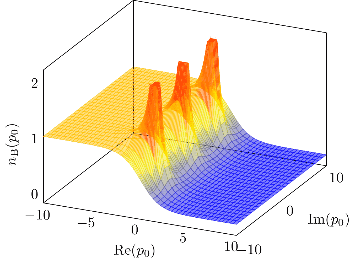
Surface plot of the Bose-Einstein distribution over the complex plane. This plot shows an important feature of the Matsubara formalism developed for QFT at non-zero temperature. It's a method to calculate expectation values of operators in a canonical ensemble evolved by an imaginary time. In momentum space, this leads to the replacement of continuous frequencies by discrete imaginary (Matsubara) frequencies. Away from the imaginary axis, the distribution becomes approximately flat, particularly at sufficiently low temperatures. Pulled from arxiv:1712.09863.
Edit
Download
Code
bose-einstein-distribution-3d.tex (34 lines)
\documentclass{standalone}

\usepackage{pgfplots,mathtools}
\pgfplotsset{compat=newest}

\let\Re\relax
\DeclareMathOperator{\Re}{Re}
\let\Im\relax
\DeclareMathOperator{\Im}{Im}

\begin{document}
\begin{tikzpicture}
  \begin{axis}[
      xlabel=$\Re(p_0)$,
      ylabel=$\Im(p_0)$,
      zlabel=$n_\text{B}(p_0)$,
      x label style={at={(0.35, 0)}},
      y label style={at={(0.95, 0.15)}},
      shader=flat,
      tickwidth=0pt
    ]

    \def\nB{(e^(2*x) - 2*e^x*cos(deg(y)) + 1)^(-1/2)}

    \addplot3[surf, opacity=0.5, domain=1:10, y domain=-10:10]{\nB};

    \addplot3[surf, opacity=0.5, domain=-10:-2, y domain=-10:10]{\nB};

    \addplot3[surf, opacity=0.5, domain=-2:1, y domain=-10:10, restrict z to domain*=0:2]{\nB};

  \end{axis}
\end{tikzpicture}
\end{document}